
Written by Sathyanarayan Rao
Introduction
Many hydrologists face the same dilemma sooner or later: do I really need a 3D model for this, or will a simple 1D line do the job? That question only makes sense once we step back and look at the bigger picture: why water management itself has become such a pressing issue. Water management has emerged as a key issue in the debate over food security as communities around the world struggle to feed an expanding population while dealing with the strains of resource scarcity, shifting land use, and climate uncertainty. Beyond agriculture, hydrology supports energy production, flood protection, urban water supply, and ecosystem preservation. However, its significance is especially apparent in agriculture. When rainfall is erratic, rivers are stressed, and groundwater supplies are depleting, it can be difficult to reliably supply crops with the water they need at the right time and location.
Here’s where hydrologic modeling comes in handy. Models enable us to forecast results, simulate various scenarios, and develop strategies that would otherwise be impossible to test on a large scale in the field by converting the complexity of water movement into organized, testable frameworks. In agriculture, this could entail determining how irrigation affects soil moisture, forecasting floodwater pooling locations on farmland, or estimating the long-term effects of groundwater extraction on crop viability. Modeling gives us the information we need to make better decisions, but it does not resolve issues on its own.
However, not all models are made equal, and their dimensionality, the amount of detail they depict is crucial. While two-dimensional methods aid in our comprehension of surface water spreading and flood hazards, a one-dimensional model might be sufficient to direct the design of an irrigation canal. The relationships between soil, groundwater, and surface water are further captured by three-dimensional models. Using my personal experience as a guide, I will discuss how the different levels of model dimensionality(1D, 2D, and 3D) apply to agriculture, although I acknowledge that the same ideas apply to a wide range of fields.
The Fundamentals of Model Dimensionality Understanding
It’s important to consider what 1D, 2D, and 3D models truly mean in hydrology before deciding when to use them.
After all, depending on gravity, soil, and pressure, water in the real world always flows sideways, downward, or upward rather than in a single direction. However, we don’t need to capture all of that complexity for a lot of real-world issues. Smart approximations that simplify the problem without sacrificing the core of the study are frequently possible.
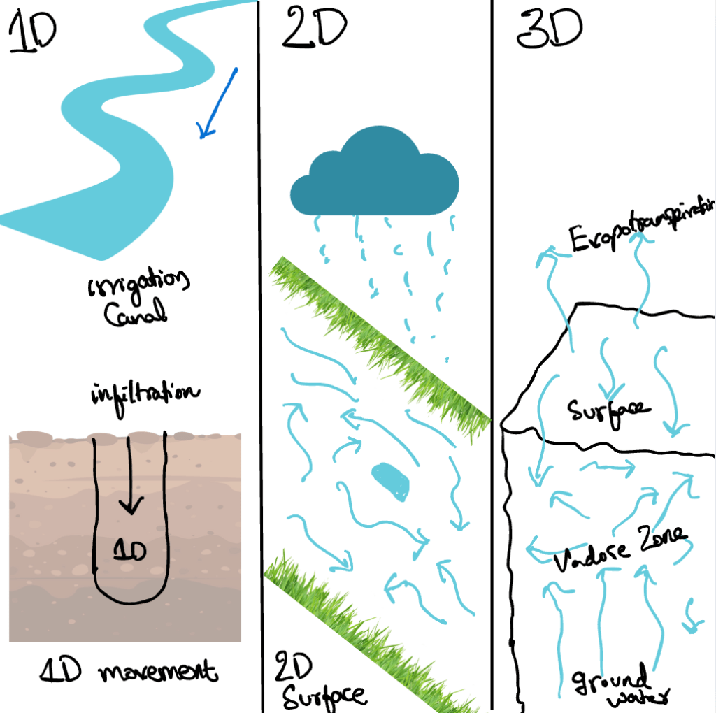
Figure 1. Conceptual illustration of dimensionality in hydrologic models. 1D captures flow along a single direction (canals, infiltration through soil layers). 2D represents water redistribution across surfaces (rainfall and runoff). 3D incorporates coupled surface–subsurface processes including evapotranspiration, vadose zone flow, and groundwater dynamics.
Consider a one-dimensional model. In actuality, soils are full of irregularities and rivers spread laterally. However, we can safely treat it as one-dimensional if the primary process of interest is water flowing through soil layers or along a channel. In order to design an irrigation canal, for instance, it is frequently necessary to model the water depth and flow rate along the channel length, which is essentially a 1D problem. Similar to this, HYDRUS-1D, which is frequently used in soil physics, illustrates the vertical infiltration and drainage of water through a soil profile. A 1D simplification saves time, data, and computing power while still providing helpful answers, even though we know that water doesn’t stay neatly in one line.
We get closer to reality with a two-dimensional model. Here, we explain how water disperses over a surface to capture patterns that are impossible for a single line to capture. When a heavy rainstorm hits farmland, the water not only sinks but also flows across the field, creating puddles in low areas and washing soil downslope. Where water will pool, how rainfall turns into runoff, or how irrigation water disperses unevenly throughout a plot can all be seen in a 2D model. These models are particularly useful for mapping floodplains, studying erosion, and creating precision irrigation systems. These surface processes are frequently simulated using programs like SWMM 2D or HEC-RAS 2D.
Last but not least, a three-dimensional model attempts to depict the entire complexity, including the vertical dimension of soil and aquifers in addition to their surface. This is important when there are groundwater-surface water interactions to consider or when processes occurring beneath the soil surface have a significant impact on surface results. For instance, a 3D representation is necessary to comprehend the amount of groundwater recharge that takes place during drip irrigation or the impact that aquifer pumping will have on river baseflow. By combining soil, groundwater, and surface hydrology, models such as MODFLOW provide information on crop water uptake, long-term sustainability, and even the movement of contaminants. Although these are effective tools, they also require a large amount of computational power and detailed data.
Therefore, dimensionality in hydrologic modeling is really about finding the ideal balance between maintaining enough realism to capture the important processes and simplifying the problem just enough to make it manageable. The decision between 1D, 2D, and 3D is based on what is practically relevant for the question we wish to answer rather than what is theoretically feasible.
1D, 2D, and 3D Hydrologic Models in Agriculture
High-performance computing and the most complex simulations are not necessary for every agricultural water issue. Sometimes all the information we require is provided by a one-dimensional model. Consider an irrigation canal’s design. How much water flows along the channel’s length and how the water depth varies as it advances are the engineer’s primary concerns. Variations from side to side are negligible and can be safely disregarded. In this instance, a 1D hydraulic model elegantly and effectively depicts fundamental physics. When examining vertical water movement through soil, the same reasoning holds true. By simulating infiltration and drainage down the profile, tools like HYDRUS-1D enable us to schedule irrigation without the need for more complex models. We would be asking the computer to solve for processes that are unrelated to the question, such as lateral spreading or intricate groundwater interactions, if we were to construct a 2D or 3D simulation here. Longer runtimes, higher data requirements, and no discernible improvement in decision accuracy would be the outcome.
Now picture an unexpected downpour over rolling farmland. Where will the rainwater go after it hits the ground? This is the practical question. Will it rush downslope and cause erosion, collect in low spots, or soak in evenly? This cannot be addressed by a one-dimensional model since it ignores the sideways spreading that in this case drives runoff and ponding and only tracks water in one direction, either down a soil profile or along a channel. Theoretically, every detail, including subsurface movement, could be represented by a three-dimensional model, but this is not necessary. We only need to understand how water redistributes itself across the field surface; we don’t need to understand the behavior of deep percolation or the interactions between groundwater and surface water. A two-dimensional model is therefore the most appropriate fit. Without wasting time and data on pointless vertical processes, it provides us with practical answers to design questions, such as where to locate erosion control structures or how to optimize a precision irrigation system, by demonstrating how topography, soil variations, and rainfall patterns control runoff. Not only is 2D more accurate than 1D in this instance, but it’s also much more efficient than going straight to 3D.
Let’s take the challenge a step further. Consider the following scenarios: how decades of groundwater pumping will impact the long-term availability of water for crops, or how much of the water applied through deep irrigation will actually replenish the aquifer during a drought. These are fundamental questions about the long-term interactions between the surface and subsurface. This cannot be addressed by a one-dimensional soil profile model since it is unable to represent the sideways flow of groundwater across the landscape and only depicts vertical movement through a soil column. The depth-dependent mechanisms that control aquifer storage, recharge, and groundwater–surface water exchange cannot be represented by a two-dimensional surface model, which is also inadequate.
Only a three-dimensional model is sufficient for this type of problem. 3D tools like MODFLOW or MIKE SHE can model the rise and fall of the groundwater table, its feedback on root-zone moisture, and even the movement of pollutants or nutrients through the soil–water system by taking into account both horizontal and vertical flow. For major decisions like groundwater sustainability studies, contamination risk assessments, and basin-scale irrigation planning, these insights are essential. Naturally, there is a cost to this: 3D models need more computing power, longer runtimes, and additional data when compared to 2D models.
In practice, hydrologists often use a mix of methods, such as 1D models for simple parts, 2D models for surface processes, and 3D models for subsurface interactions that really matter. The true test is figuring out how much complexity is too much. The next part looks at how this balance affects judgments about modeling in the real world.

Figure 2. Dimensionality in action: 1D canal flow, 2D surface redistribution (plus the occasional pond that every hydrologist dreads), and 3D groundwater flow. A reminder that no single dimension tells the whole story but together, they sketch a clearer picture.
From Conundrums to Choices: Notes on Applying Hydrologic Models
By this point, it should be clear that dimensionality is not a matter of “better” or “worse.” Each representation has its role, and in practice we rarely rely on a single model to explain an entire system. More often, hydrologists combine approaches.
Take a river valley under irrigation development. The main canals may be represented with a 1D hydraulic model to check capacity and flow distribution. A 2D surface model might then be used to examine how storm runoff spreads across floodplains. In certain sub-regions, where groundwater pumping and recharge strongly affect crops and streamflow, a 3D block is introduced. No single model could answer every part of this problem efficiently; pieced together, the results form a more coherent picture.
This hybrid way of working is increasingly common. It avoids the trap of forcing every question into a full 3D framework, which is costly and often unnecessary, while still allowing us to capture the processes that truly matter. The judgment lies in knowing which parts of a problem require higher dimensionality and which can be safely treated with simpler abstractions.
Computational realities also shape these choices. A 1D canal model can run in seconds on a standard laptop. A regional 3D groundwater–surface water simulation may demand high-memory workstations or cloud computing and can run for days. Between those extremes are many workable middle grounds. What matters is not the raw capacity of the model, but whether the results are credible given the data, the scale, and the decision at stake.
Calibration and validation are the quiet tests of all these efforts. A simple model may only need a handful of field checks; a complex 3D model demands much more extensive data collection. Either way, without careful ground-truthing, dimensionality is irrelevant.
So the choice of model is rarely about ambition. It is about sufficiency. Sometimes a single line of equations is enough; sometimes an entire 3D domain is justified. And often, the most useful answer comes from combining dimensions. Hydrologic modeling, in that sense, is not about chasing complexity but about asking good questions, staying honest about limitations, and matching the tool to the task.
Looking Ahead: Machine Learning and Emerging Tools
One reason hydrologic modeling can feel daunting is the mathematics at its core. Representing water flow through soils, rivers, and aquifers often means solving coupled partial differential equations across thousands of grid cells. For a 3D model, this process can take hours or even days, especially when repeated for calibration or scenario testing. This is where machine learning (ML) is beginning to offer a useful shortcut.
Instead of running the full physics every time, ML methods can be trained to approximate the results of a detailed model. For example, a neural network can learn the rainfall–runoff relationship from historical data, or an emulator can mimic the output of a 3D groundwater simulation in a fraction of the time. Similarly, ML can estimate difficult-to-measure parameters such as soil hydraulic properties by learning from laboratory data and extending that knowledge to field conditions. In practice, this allows hydrologists to run many more scenarios, or to bring down computational costs to something manageable on standard hardware.
This does not mean ML replaces physics. Rather, it works best in combination: physics-based models anchor our understanding, while ML fills data gaps, accelerates computation, or acts as a surrogate for costly simulations. Hybrid approaches of this kind are becoming increasingly common. They remind us that efficiency and realism do not have to compete; sometimes, the right blend of tools can provide both.
The Challenge of Uncertainty and Climate Change
An already complex field is made even more difficult by climate change. Historically, groundwater use, river regimes, and rainfall patterns have all been assumed to be somewhat stable in hydrologic models. However, those baselines are changing. Extreme events are becoming more common, aquifer demand is increasing, and rainfall has become more variable in many areas. This implies that the future may no longer be represented by the same data that was used to calibrate earlier models.
This creates an uncertainty problem for modelers. When the future climate itself is uncertain, how do we choose a model dimensionality? Investigating a larger range of scenarios has been one response. Broad risks and trends can be identified by screening a large number of potential futures using simpler models that are quicker to run and simpler to calibrate. The most crucial situations, where a high degree of confidence is necessary for decision-making, are then tested using more intricate 3D models.
This two-pronged strategy strikes a balance between depth and speed. It acknowledges that while uncertainty cannot be completely eradicated, it can be mapped out and comprehended. Even in the face of changing climate conditions, hydrologists can stress-test agricultural water systems against drought, flooding, and long-term groundwater depletion by combining models with varying dimensionalities. Predicting a single, precise result is less of a challenge than being ready for a variety of scenarios in a world that is changing.
Conclusion: A Note to Early-Career Hydrologists
For those entering the field, the temptation will always be to reach for the most detailed model, the latest software, or the largest dataset. But hydrologic modeling is less about chasing complexity and more about asking good questions. A simple 1D model, well-calibrated, can sometimes provide more clarity than a sprawling 3D system run on borrowed supercomputers. At the same time, there will be moments when nothing short of a 3D representation will do.
What matters is learning to match the tool to the task, being transparent about limitations, and remembering that models are approximations of a world more complex than any grid or equation can fully capture. As climate pressures grow and new technologies like machine learning expand our options, this humility becomes even more important.
So, start with the fundamentals. Build familiarity with 1D and 2D methods before stepping into 3D. Explore hybrid approaches where different tools complement each other. Stay curious about emerging techniques, but ground them in physics and data. Above all, keep in mind that the value of a model is not in its dimensionality or sophistication, but in the decisions it helps us make more responsibly.
Hydrology will always be part science, part pragmatism. For young hydrologists, the real skill lies in balancing those parts with patience, honesty, and care.
About the author
Sathyanarayan Rao is a Research Associate at the Indian Institute of Science, Bengaluru and is a YHS blog committee member. He completed his PhD in Engineering Sciences at UCLouvain, Belgium in 2020, where he worked on computational modeling of the electrical signatures of plant roots as part of the eRoot project. His research interests span soil-root water modeling, digital twins in agriculture, and scientific computing. Over the years, Rao has had the opportunity to work across institutions in India, Europe, and the USA, contributing to topics ranging from root phenotyping to computational physics. Beyond research, he is a passionate science communicator and hobby writer. He enjoys creating educational content on the internet. In his free time, you’ll often find him exploring new places—traveling is a hobby that keeps him inspired. He can be reached at satraox@gmail.com
